
| 일 | 월 | 화 | 수 | 목 | 금 | 토 |
|---|---|---|---|---|---|---|
| 1 | 2 | 3 | 4 | 5 | ||
| 6 | 7 | 8 | 9 | 10 | 11 | 12 |
| 13 | 14 | 15 | 16 | 17 | 18 | 19 |
| 20 | 21 | 22 | 23 | 24 | 25 | 26 |
| 27 | 28 | 29 | 30 |
Tags
- regression
- pytorch
- mnist
- 파이토치
- 딥러닝
- 파이토치로 시작하는 딥러닝 기초
- 로보틱스 입문
- 로보틱스입문
- Numpy
- DeepLearning
- pytorch visdom
- Introduction to Robotics: Mechanics and Control by John J Craig
- Robotics
- Robot arm
- Python
- softmax
- visdom
- DH parameter
- dynamixel
- custom cnn
- boostcourse
- Pytorch로 시작하는 딥러닝 입문
- IMU sensor
- nucleo-f401re
- 6dof
- RobotArm
- 6축 다관절
- PUMA 560
- NUCLEO board
- 6자유도 로봇팔
Archives
- Today
- Total
슬.공.생
BoostCourse(DL)(week1)-Multi_Linear_Regerssion 본문
study/DeepLearning
BoostCourse(DL)(week1)-Multi_Linear_Regerssion
AGT (goh9510@naver.com) 2022. 7. 25. 20:46본 포스팅은 부스트 코스의 [파이토치로 시작하는 딥러닝 기초]를 수강하며 진행한 내용 정리입니다
파이토치로 시작하는 딥러닝 기초
부스트코스 무료 강의
www.boostcourse.org
본 글은 선형 회귀와 해당 실습을 정리하기 위해 작성되었습니다.
선형 회귀란?
- 학습 데이터들과 가장 유사한 값을 가지는 데이터들을 하나의 직선으로 표현한 것이다.
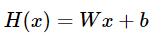
- 표현이 직선이기 때문에 선형 회귀는 위와 같은 1차 함수 형태의 가설 함수(Hypothesis)를 사용하게 된다.
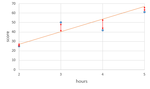
- 훈련 데이터 들과 위의 식의 값들을 비교하며 (W)와 (b) 값들을 점진적으로 수정하게 되며
- 가설 함수와 실제 값들의 오차(error OR cost)를 최소화하는 방향으로 반복 과정 거치게 된다.
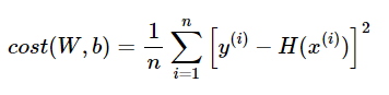
- 실제 훈련 결과 데이터인 y, 가설 함수의 결괏값인 H를 비교하여 cost 값을 만들면 출력은 cost, 입력은 W, b인 아래와 같은 2차 함수가 된다.
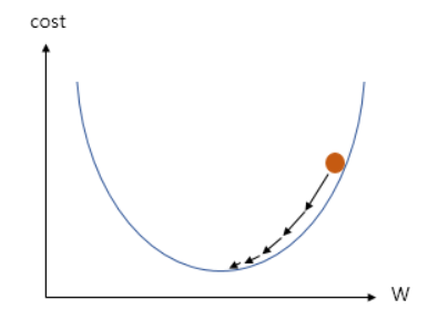
- cost(error)를 최소화시키는 방향으로 W, b를 찾는것이 목적이므로 위 그래프의 출력의 최소지점인 기울기(순간변화율이)가 0인 지점의 W,b를 찾아낸다.
- 이때 사용되는 것이 Gradient decent이다
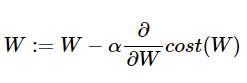
- 위의 식처럼 각각 지점에서 W에 대한 cost함수의 미분 값을 이용, 적절한 상수값을 곱하여 새로운 W 값을 만들어 내게 된다.
- 기울기가 0인 지점을 기준으로 삼는다면, 기준점으로 부터 멀리 있는 부분에서는 큰 기울기가, 가까운 부분에서는 작은 기울기가 계산될 것이다.
- 기준점으로부터의 거리에 비례하여서 W값이 변해야 하는 값도 결정된다. 따라서 각 지점의 기울기 값을 이용하여 기준점(기울기 0)으로 근접해 나갈 수 있다.
- 위의 과정을 반복하고 cost가 최소화되는 지점의 W, b값을 찾으며 선형 회귀가 진행된다.
아래는 실제 코드를 작성해보며 실습한 내용이다
- 다중 입력 선형 회귀를 위해 아래와 같이 x_train, y_train을 구성한다. 입출력 = (3, 1)
import torch
import torch.nn as nn
import torch.nn.functional as F
import torch.optim as optim

torch.manual_seed(1)

## train data
x_train  = torch.FloatTensor([[73, 80, 75],
                              [93, 88, 93],
                              [89, 91, 90],
                              [96, 98, 100],
                              [73, 66, 70]])
y_train = torch.FloatTensor([[152], [185], [180], [196], [142]])
- 다중 입력의 경우 weight(W)와 bias(b)를 각각 선언해 주어야 한다.
- 각각 선언하는 방식 대신 nn.module을 상속받는 class 선언을 통해 다중 입력 선형회귀 객체(모델을)를 만들도록 구성한다.
## model = nn.Linear(1,1)
## class로 model 입출력 선언??
class MultivariateLinearRegressionModel(nn.Module):
    def __init__(self):
        super().__init__()
        self.linear = nn.Linear(3, 1)

    def forward(self, x):
        return self.linear(x)


model = MultivariateLinearRegressionModel()


## print(x_train, y_train)
##모델 준비 및 초기화

##W = torch.zeros((3, 1), requires_grad = True)
##b = torch.zeros(1, requires_grad=True)
## requires_grad 라는것은 학습되어 값이 바뀔 대상이라는 뜻
- model의 parameter를 통해 weights, bias를 optimizer에 전달한다.
##optimizer 설정
##optimizer = torch.optim.SGD([W, b], Ir = 0.000001)
optimizer = torch.optim.SGD(model.parameters(), lr=0.00001)
- x_train data가 다중입력 data 로서 W[]와 연산을 위해 matmul()을 사용하여 Hypothesis를 구성한다.
nb_epochs = 200
for epoch in range(nb_epochs +1 ):

    ##hypothesis = x_train.matmul(W) + b
    hypothesis = model(x_train)

    ##cost = torch.mean((hypothesis - y_train)**2)
    cost = F.mse_loss(hypothesis, y_train)

    ##gradient 초기화
    optimizer.zero_grad()
    ## cost 값으로 hypothesis 지속적으로 수정
    cost.backward()
    optimizer.step()

    print('Epoch {:4d}/{} hypothesis: {} Cost: {:.6f}'.format(
        epoch, nb_epochs, hypothesis.squeeze().detach(),
        cost.item()

))'study > DeepLearning' 카테고리의 다른 글
| BoostCourse(DL)(week2)-Sequential model(class) (0) | 2022.08.01 |
|---|---|
| BoostCourse(DL)(week2)-Logistic Regression (0) | 2022.08.01 |
| BoostCourse(DL)(week1)-Mini Batch Gradient Descent (0) | 2022.07.30 |
| BoostCourse(DL)(week1)-class 기반 모델 구현(보충) (0) | 2022.07.30 |
| BoostCourse(DL)(week1)-Tensor Manipulation (0) | 2022.07.24 |
'study/DeepLearning' Related Articles
more


Comments